Extending Factor¶

Rethink NormalData¶

Normal data format is as below:

Why use this format?

The reason is that human is comfortable for two-dimensional space and high-dimensional space could be reduced to it.

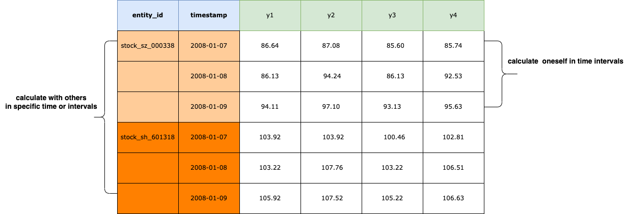
Obviously, It’s complete and consistent. You could calculate oneself in time intervals or calculate with others in specific time or intervals. And it’s easy to analyze the data with charts by Intent.

Factor data structure¶

The factor computing flow is as below:

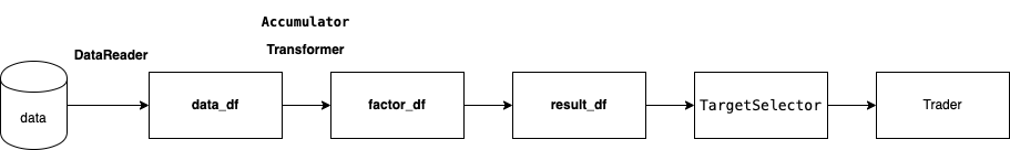
data_df

NormalData df read from the schema.

factor_df

NormalData df computed by data_df using use Transformer, Accumulator or your custom logic.

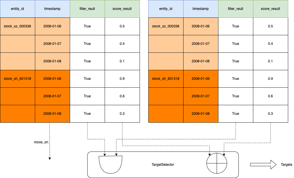
result_df

NormalData df containing columns filter_result and(or) score_result which calculated using factor_df or(and) data_df. Filter_result is True or False, score_result is from 0 to 1. You could use TargetSelector to select targets at specific time when filter_result is True and(or) score_result >=0.8 by default or do more precise control by setting other arguments.

Let’s take BullFactor to illustrate the calculation process:

>>> from zvt.factors.macd import BullFactor
>>> from zvt.domain import Stock1dHfqKdata
>>> entity_ids = ["stock_sh_601318", "stock_sz_000338"]
>>> Stock1dHfqKdata.record_data(entity_ids=entity_ids, provider="em")
>>> factor = BullFactor(entity_ids=entity_ids, provider="em", start_timestamp='2019-01-01', end_timestamp='2019-06-10')

check the dfs:

>>> factor.data_df
>>> factor.factor_df
>>> factor.result_df

Write transformer¶

Transformer works as bellow:

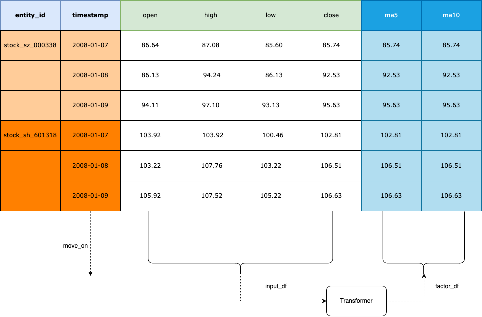
What’s in your mind is the NormalData format, and then practice the skills to manipulate it.

You could use other ta lib with it easily, e.g Bollinger Bands using TA lib

install ta at first:

pip install --upgrade ta

write boll transformer and factor:

from typing import Optional, List

import pandas as pd
from ta.volatility import BollingerBands

from zvt.contract.factor import *
from zvt.factors import TechnicalFactor


class BollTransformer(Transformer):
    def transform_one(self, entity_id, df: pd.DataFrame) -> pd.DataFrame:
        indicator_bb = BollingerBands(close=df["close"], window=20, window_dev=2)

        # Add Bollinger Bands features
        df["bb_bbm"] = indicator_bb.bollinger_mavg()
        df["bb_bbh"] = indicator_bb.bollinger_hband()
        df["bb_bbl"] = indicator_bb.bollinger_lband()

        # Add Bollinger Band high indicator
        df["bb_bbhi"] = indicator_bb.bollinger_hband_indicator()

        # Add Bollinger Band low indicator
        df["bb_bbli"] = indicator_bb.bollinger_lband_indicator()

        # Add Width Size Bollinger Bands
        df["bb_bbw"] = indicator_bb.bollinger_wband()

        # Add Percentage Bollinger Bands
        df["bb_bbp"] = indicator_bb.bollinger_pband()
        return df


class BollFactor(TechnicalFactor):
    transformer = BollTransformer()

    def drawer_factor_df_list(self) -> Optional[List[pd.DataFrame]]:
        # set the factor to show
        return [self.factor_df[["bb_bbm", "bb_bbh", "bb_bbl"]]]

    def compute_result(self):
        # set filter_result, which bb_bbli=1.0 buy and bb_bbhi=1.0 sell
        super().compute_result()
        self.result_df = (self.factor_df["bb_bbli"] - self.factor_df["bb_bbhi"]).to_frame(name="filter_result")
        self.result_df[self.result_df == 0] = None
        self.result_df[self.result_df == 1] = True
        self.result_df[self.result_df == -1] = False

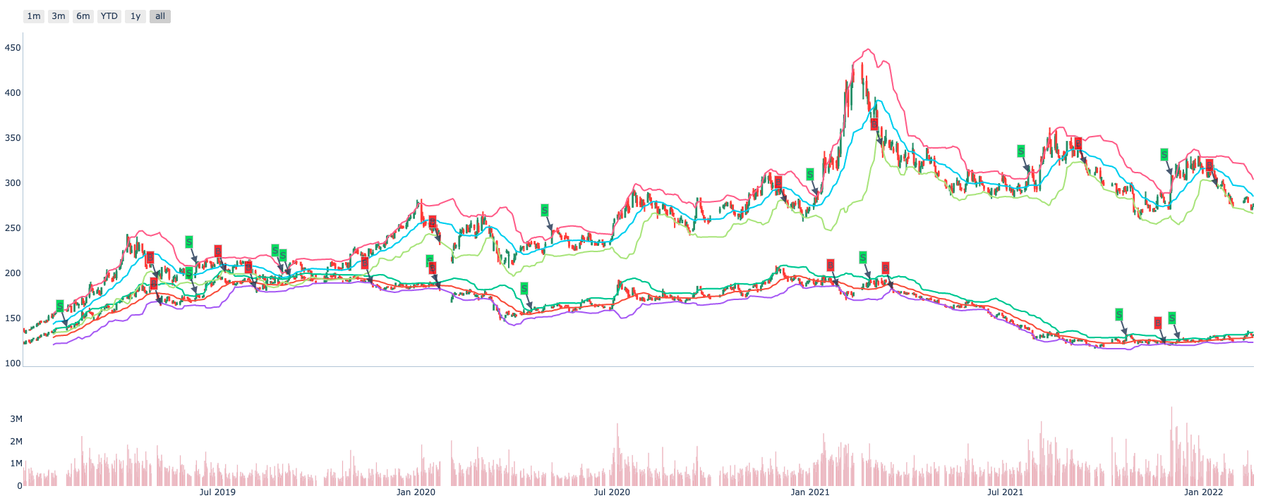
Let’s show it:

>>> from zvt.domain import Stock1dHfqKdata

>>> provider = "em"
>>> entity_ids = ["stock_sz_000338", "stock_sh_601318"]
>>> Stock1dHfqKdata.record_data(entity_ids=entity_ids, provider=provider,)
>>> factor = BollFactor(
>>> entity_ids=entity_ids, provider=provider, entity_provider=provider, start_timestamp="2019-01-01"
>>> )
>>> factor.draw(show=True)

Most of ta lib support calculate single target by default, so we implement transform_one of the Transformer. If you want to calculate many targets at the same time you could implement transform directly and it would be faster.

And Transformer is stateless, so it’s easy to reuse in different factor if need.

Factor with IntervalLevel¶

After you write the transformer and construct the factor, it’s easy to use in different levels.

Let’s use BollFactor in IntervalLevel 30m:

>>> from zvt.domain import Stock30mHfqKdata

>>> provider = "em"
>>> entity_ids = ["stock_sz_000338", "stock_sh_601318"]

>>> Stock30mHfqKdata.record_data(entity_ids=entity_ids, provider=provider)
>>> factor = BollFactor(
        entity_ids=entity_ids, provider=provider, entity_provider=provider, start_timestamp="2021-01-01"
    )
>>> factor.draw(show=True)

Stream computing¶

The data is coming continuously and the factor using the data need computing continuously too.

It’s simple and straightforward:

{Schema}.record_data in one process
{Factor}.move_on which call {Schema}.query_data in another process

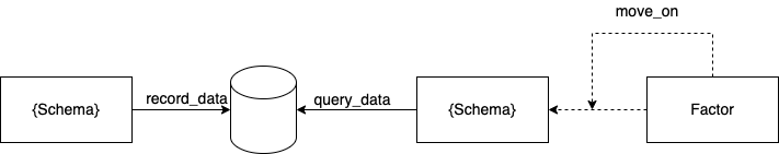
We keep the simple enough philosophy: single process and thread. Enjoy programming and make everything clear.

Factor persistence¶

Getting data and computing factor continuously is cool. But…If It took a long time to calculate the factor and crashed.How would you feel?

Select the targets¶

You could select the targets according result_df of the factor by yourself. Or use TargetSelector do it for you.

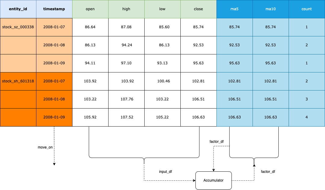
Write accumulator¶